Getting Started with aimsprop🔗

What is aimsprop?🔗

This package was developed to analyse data from AIMS simulations. The functionality revolves around a Bundle object which properties can be calculated on, for example geometric properties, time dependent spectra, population decay etc. The Bundle object consists of a list of Frame objects, which contain the properties.

The documentation for the package can be found here.

Creating a Bundle object from an AIMS run🔗

First, make sure that you have the package installed: pip install aimsprop

Then you can import the package into your file:

import aimsprop as ai

The documentation for creating and manipulating bundle objects can be found here.

You can read in an AIMS simulation from and FMS90 run. As an example, we will read in the data used for testing, so we set aims_dir = "tests/test_data/" and we set IC = "0002". These should be changed to the path to your AIMS output.

First, to create a Path object to the AIMS data (this is better than using a simple string since it manages file/dir paths well).

from pathlib import Path

aims_path = Path(aims_dir)

We can then pass the Path object into aimsprop:

bundle = ai.parse_fms90(aims_path / IC, scheme='mulliken')

We can also read in a collection AIMS runs from different initial conditions. We can set ICs = ["0002","0003"]:

bundles = [ai.parse_fms90(aims_path / IC, scheme='mulliken') for IC in ICs]

Here, the variable bundles is a list of Bundle objects which can be merged together to form the AIMS simulation, containing the data for all the specified initial conditions. The weights of each bundle are specified, which can be set according to the IC oscillator strength or the ICs can be weighted evenly as below:

simulation = ai.Bundle.merge(bundles, ws=[1.0 / len(bundles)] * len(bundles), labels=ICs)

If you have terminated your TBFs on the ground state and run adiabatic extensions, you can pass the xyz files from these using ai.parse_xyz. The time should be set to when the ground state TBF begins and then this can be merged into simulation for the IC it is associated with using the ai.Bundle.merge function as above.

Cleaning the simulation🔗

FMS90 AIMS simulations include adaptive time steps in regions of high non-adiabatic coupling. It is often useful to remove these adaptive timesteps and have evenly spaced time steps for your Bundle object. First we can define the times that we want our Bundle frames to be, e.g. ts = np.arange(0.0, max(simulation.ts), 40.0).

simulation = simulation.interpolate_linear(ts)

We can also remove duplicates incase any exist, e.g. from AIMS restarts:

simulation = simulation.remove_duplicates()

Using the Bundle object🔗

As noted previously, the Bundle object consists of a list of Frame objects. Therefore you can iterate through the frames and print or extract frame properties:

for frame in simulation.frames:
    label = frame.label
    time = frame.t
    weight = frame.w
    state = frame.I
    widths = frame.widths

You can also extract the list of properties for the entire Bundle simulation using, for example:

labels = simulation.labels
times = simulation.ts
weights = simulation.ws
states = simulation.Is

You can select only a portion of the total simulation using the subset_by_<> functions:

simulation_s0 = simulation.subset_by_I(1)
simulation_500au = simulation.subset_by_t(500)

Computing geometric properties🔗

The geometric properties that are supported are:

Bond length
Bond angle
Torsion angle
Out of plane angle
Proton transfer coordinate.

The documentation for the geometric functions can be found here.

Bond length🔗

You can calculate the bond length between two atoms, e.g atom indices 0 and 1 and name the property, e.g. "R01":

ai.compute_bond(simulation, "R01", 0, 1)

Bond angle🔗

You can calculate the bond angle between three atoms, e.g atom indices 0, 1 and 2 name the property, e.g. "A012":

ai.compute_angle(simulation, "A012", 0, 1, 2)

Torsion angle🔗

You can calculate the torsion angle between four atoms, e.g atom indices 0, 1, 2 and 3 and name the property, e.g. " T0123":

ai.compute_torsion(simulation, "T0123", 0, 1, 2, 3)

You can also unwrap properties so that it continues beyond 180 degrees rather than jumping back down to -180:

ai.unwrap_property(simulation, "T0123", 360.0)

Transfer coordinate🔗

You can calculate the transfer coordinate between atoms, e.g atom indices 0, 1, and 2 and name the property, e.g. "PT012":

ai.compute_transfer_coord(simulation, "PT012", 0, 1, 2)

Extracting properties🔗

Once a property has been added to the Bundle object, it can be extracted with its key id:

r01 = simulation.extract_property("R01")

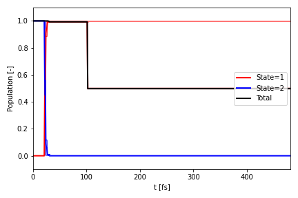
Calculate Population🔗

Documentation for the population can be found here.

If you want to calculate the population use

pop = ai.compute_population(simulation)

If you just want to plot the population to a file, e.g. P.png, you can instead run:

ai.plot_population(
    "P.png",
    simulation,
    bundles,
    time_units="fs",
    state_colors=["r", "b"],
)

where simulation is the merged Bundle object, and bundles is the list of parsed Bundle objects. The file can also be saved as a PDF or PNG.

Plotting properties🔗

Documentation for the plotting functions can be found here.\ You can plot scalar properties and blurred properties. The files can be written as PNG or PDF files.

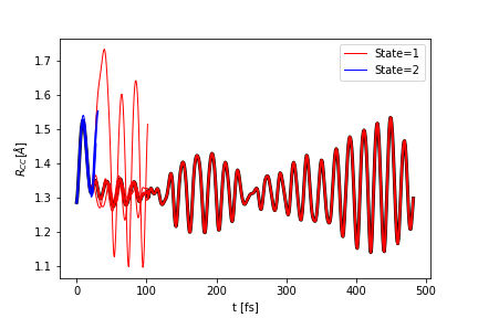
Plot scalar properties🔗

You can plot the properties that you calculated above, for example plotting the bond angle:

ai.plot_scalar("R.png",
               simulation,
               "R01",
               ylabel=r"$R_{CC} [\AA{}]$",
               time_units="fs",
               state_colors=["r", "b"],
               clf=False,
               plot_average=True,
               )

The figure is saved to the file R.png. The function returns the plt object so it can be modified as needed.

Plot vector properties🔗

The documentation for applying a Gaussian to a property is here.

In order to blur a property using a Gaussian convolution, first create a space over which the property can be blurred, and then computer the blurred property:

R = np.linspace(0, 7, 100)
ai.blur_property(simulation, "R01", "R01blur", R, alpha=8.0)

The blurred property is written with key, "R01blur".

To plot a blurred property use:

ai.plot_vector(
    "Rblur.png",
    simulation,
    "R01blur",
    y=R,
    ylabel=r"$R [\AA{}]$",
    time_units="fs",
    nlevel=64
)

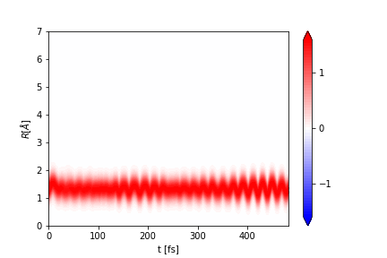
The figure is saved to the file Rblur.png. The function returns the plt object, so it can be modified as needed.

The same can be done for the other properties.

Time dependent spectra🔗

Currently, ultrafast electron diffraction and ultrafast x-ray scattering signals can be computed with aimsprop.\ There is more information on these techniques here.

Ultrafast electron diffraction🔗

The Ultrafast electron diffraction (UED) signal can be generated by defining a bond length range and then computing the signal:

R = np.linspace(1.0, 6.0, 50)
ai.compute_ued_simple(simulation, "UED", R=R, alpha=8.0)

Notes on how the UED signal is computed can be found here.

You can then plot the signal:

ai.plot_vector(
    "UED.png",
    simulation,
    "UED",
    y=R,
    ylabel=r"$R [\AA{}]$",
    time_units="fs",
    diff=True
)

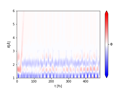
The figure will be saved in UED.png.

Reading and Writing Bundle objects🔗

You can use pickle to write/read in the Bundle object so you dont have to re-generate it again each time.

First, load pickle:

import pickle

Writing the Bundle object simulation to a file:

with open("simulation.out", "wb") as f:
    pickle.dump(simulation, f)

Reading it back from a file:

with open("simulation.out", "rb") as f:
    simulation = pickle.load(f)

When the Bundle object is written to a file, all of its properties are also written. Therefore when it is read from a pickle file, it contains all information that was stored in it, including its properties.

Writing xyz files🔗

The documentation for xyz files can be found here. You can parse xyz files into aimsprop to build a Bundle object. You can also write them:

ai.write_xyzs(simulation, ".")